Smoothing techniques: Difference between revisions
Bosmana fem (talk | contribs) |
Bosmana fem (talk | contribs) |
||
| (2 intermediate revisions by the same user not shown) | |||
| Line 20: | Line 20: | ||
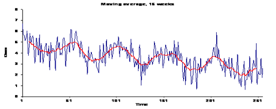
Figure 3: Crude data, and 15 weeks moving average | Figure 3: Crude data, and 15 weeks moving average | ||
[[File: | [[File:seasonality.png|600px|frame|none]] | ||
Principles for calculating moving averages | Principles for calculating moving averages | ||
| Line 47: | Line 47: | ||
|} | |} | ||
Using the median value over the window rather than the mean generates a moving median | Using the median value over the window rather than the mean generates a moving median that is more robust to outliers than the mean. In such case, the Excel © formula should be =MEDIAN(B2:B6) in cell C4 and copied over the range. Note that functions in MS-Excel© may vary according to language. | ||
<div style="display: inline-block; width: 25%; vertical-align: top; border: 1px solid #000; background-color: #d7effc; padding: 10px; margin: 5px;"> | |||
'''FEM PAGE CONTRIBUTORS 2007''' | |||
;FEM Editor 2007 | |||
:Denis Coulombier | |||
;Original FEM Authors | |||
:Christophe Paquet | |||
:Arnold Tarantola | |||
:Philippe Quenel | |||
:Nada Ghosn | |||
;FEM Contributors | |||
:Denis Coulombier | |||
:Lisa Lazareck | |||
:Vladimir Prikazsky | |||
</div> | |||
[[Category:Analysis by time characteristics]] | |||
Latest revision as of 21:57, 10 April 2023
Plotting crude data
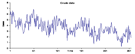
Visual exploration of a time series uses a graphical presentation of the data plotted along a time axis. The graph must be as simple as possible to allow a good visual inspection of the data.
Figure 1: Crude data signal
The descriptive analysis of a time series aims to characterize it in terms of trends and seasons.
Describing a trend
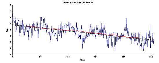
Describing a trend requires a moving average window encompassing a full year (i.e. 52 weeks for weekly data). The shape of the resulting trend line is visually compared to the linear regression line.
Figure 2: Crude data, 52 weeks moving average, and a regression line
Describing seasonal variations
A moving average window of 15 weeks smoothes the crude series, highlighting the seasonal pattern of the series. The size of the moving average windows depends upon the variance of the series, corresponding to the amount of variability to be smoothed. In general, windows from 5 to 15 weeks result in appropriate smoothing, but visual inspection of the result is required.
Figure 3: Crude data, and 15 weeks moving average
Principles for calculating moving averages Spreadsheet software such as Microsoft Excel © allows to easily display time series filtered by a moving average window. For description purposes, it is important to display the averaged value in the center of the moving average window. The example below used a five-week moving average window. The first value equals the sum of the first 5 weeks, divided by 5 (5.73). This value is plotted against week 3, which represents the middle week for this first window.
Table 1: Crude series, formulas and smoothed series for calculating moving averages in Excel (5 week window)
| A | B | C | D |
|---|---|---|---|
| 1 | Time | Crude data | Formulas |
| 2 | 1 | 6.70 | |
| 3 | 2 | 5.73 | |
| 4 | 3 | 5.59 | 2,5 |
| 5 | 4 | 5.15 | 3 |
| 6 | 5 | 5.47 | 4 |
| 7 | 6 | 6.03 | 5 |
| 8 | 7 | 3.75 | 5,5 |
Using the median value over the window rather than the mean generates a moving median that is more robust to outliers than the mean. In such case, the Excel © formula should be =MEDIAN(B2:B6) in cell C4 and copied over the range. Note that functions in MS-Excel© may vary according to language.
FEM PAGE CONTRIBUTORS 2007
- FEM Editor 2007
- Denis Coulombier
- Original FEM Authors
- Christophe Paquet
- Arnold Tarantola
- Philippe Quenel
- Nada Ghosn
- FEM Contributors
- Denis Coulombier
- Lisa Lazareck
- Vladimir Prikazsky


