Linear models: Difference between revisions
Bosmana fem (talk | contribs) |
Bosmana fem (talk | contribs) |
||
| (5 intermediate revisions by the same user not shown) | |||
| Line 2: | Line 2: | ||
Mathematical models can be as simple as a straight line. In a linear model the straight line is used to describe the relation between two variables. We express y according to the value of x. We predict y according to x. Therefore x is called the predictor or independent variable and y the predicted or dependent variable. | Mathematical models can be as simple as a straight line. In a linear model the straight line is used to describe the relation between two variables. We express y according to the value of x. We predict y according to x. Therefore x is called the predictor or independent variable and y the predicted or dependent variable. | ||
[[File:3240.Straight.gif-550x0.png|600px|frameless|centre|Figure 1 shows the relation between y and x]] | |||
[[File:3240.Straight.gif-550x0.png| | Figure 1 shows the relation between y and x | ||
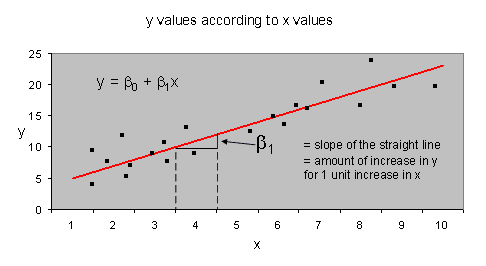
The straight line represents the average values of y for different values of x. It is a regression line. It was obtained by fitting a straight line equation to the data. A simple way to understand how the straight line is fitted on the dot plot is to visually guess where it would need to be placed in order to minimise the various distances between each dot and the line. | The straight line represents the average values of y for different values of x. It is a regression line. It was obtained by fitting a straight line equation to the data. A simple way to understand how the straight line is fitted on the dot plot is to visually guess where it would need to be placed in order to minimise the various distances between each dot and the line. | ||
| Line 10: | Line 9: | ||
The equation of a straight line is: | The equation of a straight line is: | ||
y = β0 + β1x | y = β0 + β1x | ||
In which | In which | ||
| Line 27: | Line 26: | ||
The coefficients β1 and β2 respectively provide estimate of the effect of x1 and x2 which are mutually un-confounded. Mathematically there are no limits to the number of variables to be included in a model. | The coefficients β1 and β2 respectively provide estimate of the effect of x1 and x2 which are mutually un-confounded. Mathematically there are no limits to the number of variables to be included in a model. | ||
<div style="display: inline-block; width: 25%; vertical-align: top; border: 1px solid #000; background-color: #d7effc; padding: 10px; margin: 5px;"> | |||
'''FEM PAGE CONTRIBUTORS 2007''' | |||
;Editor | |||
: Fernando Simon | |||
;Original Author | |||
: Alain Moren | |||
;Contributors | |||
: Arnold Bosman | |||
: Lisa Lazareck | |||
: Fernando Simon | |||
</div> | |||
[[Category:Logistic Regression]] | [[Category:Logistic Regression]] | ||
Latest revision as of 21:47, 10 April 2023
The straight line
Mathematical models can be as simple as a straight line. In a linear model the straight line is used to describe the relation between two variables. We express y according to the value of x. We predict y according to x. Therefore x is called the predictor or independent variable and y the predicted or dependent variable.
Figure 1 shows the relation between y and x
The straight line represents the average values of y for different values of x. It is a regression line. It was obtained by fitting a straight line equation to the data. A simple way to understand how the straight line is fitted on the dot plot is to visually guess where it would need to be placed in order to minimise the various distances between each dot and the line.
The equation of a straight line is:
y = β0 + β1x
In which
β0 is the intercept (value of y when x = 0)
β1x is the coefficient of x. It describes the slope of the line. It represents the number of units of change in y when x increases by 1 unit.
The general linear model
Let's suppose that in the above example we want to predict y not only according to x1 but also according to x2. We would have then two predictors. The relation between x1 , x2 and y is still a straight line. The equation is now:
y = β0 + β1x1 + β2x2
To locate the straight line in the dots we need to imagine a 3 dimensional rectangle coordinates with y expressed according to x1 and x2.
The coefficients β1 and β2 respectively provide estimate of the effect of x1 and x2 which are mutually un-confounded. Mathematically there are no limits to the number of variables to be included in a model.
FEM PAGE CONTRIBUTORS 2007
- Editor
- Fernando Simon
- Original Author
- Alain Moren
- Contributors
- Arnold Bosman
- Lisa Lazareck
- Fernando Simon
