The logistic model: Difference between revisions
Bosmana fem (talk | contribs) mNo edit summary |
Bosmana fem (talk | contribs) |
||
| (6 intermediate revisions by the same user not shown) | |||
| Line 1: | Line 1: | ||
In the linear model y can take all possible values from - ∞ to + ∞. However in epidemiology we are mainly interested in binary outcomes (ill or not, dead or not, etc.). They are frequently noted as 0 and 1. | In the linear model y can take all possible values from - ∞ to + ∞. However in epidemiology we are mainly interested in binary outcomes (ill or not, dead or not, etc.). They are frequently noted as 0 and 1. | ||
[[File:4174.CHD dicotomous.gif-550x0.png|600px|frameless|center]] | |||
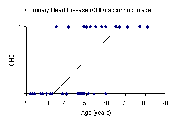
Figure 1 shows the hypothetical distribution of cases of coronary heart disease (CHD) according to age. | Figure 1 shows the hypothetical distribution of cases of coronary heart disease (CHD) according to age. | ||
From the above graph it seems that CHD cases may be older than others. A regression line would not really reflect the relation. In addition y, being a straight line, could vary between - ∞ and + ∞ which is not what we expect for disease occurence. | From the above graph it seems that CHD cases may be older than others. A regression line would not really reflect the relation. In addition y, being a straight line, could vary between - ∞ and + ∞ which is not what we expect for disease occurence. | ||
| Line 62: | Line 61: | ||
[[File: | [[File:3326.image007.gif-550x0.png|600px|frameless|center]] | ||
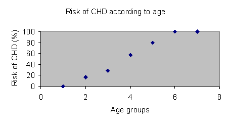
Figure 2: Proportion of persons at risk of CHD by age group | Figure 2: Proportion of persons at risk of CHD by age group | ||
Therefore we would be interested in identifying a transformation of the linear model which would limit the value of y between 0 and 1 in order to avoid getting impossible values for y. | Therefore we would be interested in identifying a transformation of the linear model which would limit the value of y between 0 and 1 in order to avoid getting impossible values for y. | ||
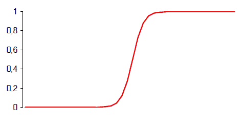
The logistic function which is "S " shaped satisfies those constraints (figure 3). | The logistic function which is "S " shaped satisfies those constraints (figure 3). | ||
[[File:6708.Logistic.gif-550x0.png|600px|frameless|center]] | |||
Figure 3: The logistic function | |||
The logistic function that we will use in logistic regression can be written as follows: | The logistic function that we will use in logistic regression can be written as follows: | ||
[[File:3302.image011.gif-550x0.png|600px|frameless|center]] | |||
R (the risk) is also frequently noted as P (y/x) which is the probably of the outcome given x. In that case the above formula is: | R (the risk) is also frequently noted as P (y/x) which is the probably of the outcome given x. In that case the above formula is: | ||
[[File:5556.image013.gif-550x0.png|600px|frameless|center]] | |||
| Line 96: | Line 93: | ||
One of the major advantages of multivariable analysis is that it will allow controlling of confounding simultaneously in all variables included in a model. Variables would be then mutually unconfounded. | One of the major advantages of multivariable analysis is that it will allow controlling of confounding simultaneously in all variables included in a model. Variables would be then mutually unconfounded. | ||
<div style="display: inline-block; width: 25%; vertical-align: top; border: 1px solid #000; background-color: #d7effc; padding: 10px; margin: 5px;"> | |||
'''FEM PAGE CONTRIBUTORS 2007''' | |||
; Editor | |||
: Fernando Simon | |||
;Original Author | |||
: Alain Moren | |||
; Contributors | |||
: Arnold Bosman | |||
: Lisa Lazareck | |||
: Fernando Simon | |||
</div> | |||
[[Category:Logistic Regression]] | [[Category:Logistic Regression]] | ||
Latest revision as of 21:15, 10 April 2023
In the linear model y can take all possible values from - ∞ to + ∞. However in epidemiology we are mainly interested in binary outcomes (ill or not, dead or not, etc.). They are frequently noted as 0 and 1.
Figure 1 shows the hypothetical distribution of cases of coronary heart disease (CHD) according to age.
From the above graph it seems that CHD cases may be older than others. A regression line would not really reflect the relation. In addition y, being a straight line, could vary between - ∞ and + ∞ which is not what we expect for disease occurence.
In the following table and figure, the relation between age and CHD is expressed as the proportion of persons with CHD (risk) by 10 years age groups. The increase of risk of CHD with age is clearer and risk goes from 0 to 1 (here expressed as a %).
Table 1: Proportion of persons at risk of CHD by age group
| Age group | Age group in years | Number in group | Disease | Proportion % |
|---|---|---|---|---|
| 1 | 20-29 | 5 | 0 | 0 |
| 2 | 30-39 | 6 | 1 | 17 |
| 3 | 40-49 | 7 | 2 | 29 |
| 4 | 50-59 | 7 | 4 | 57 |
| 5 | 60-69 | 5 | 4 | 80 |
| 6 | 70-79 | 2 | 2 | 100 |
| 7 | 80+ | 1 | 1 | 100 |
Figure 2: Proportion of persons at risk of CHD by age group
Therefore we would be interested in identifying a transformation of the linear model which would limit the value of y between 0 and 1 in order to avoid getting impossible values for y.
The logistic function which is "S " shaped satisfies those constraints (figure 3).
Figure 3: The logistic function
The logistic function that we will use in logistic regression can be written as follows:
R (the risk) is also frequently noted as P (y/x) which is the probably of the outcome given x. In that case the above formula is:
The logistic function needs to be transformed to become a user friendly tool. The transformation will help us keeping the values in the appropriate range. The logistic transformation includes two steps. The first is to use the odds of disease (P(y/x) / (1- P(y/x)) instead of the risk (P(y/x)). The second transformation is to take the natural logarithm of the odds of disease, ln [ (P(y/x) / (1- P(y/x)]. The result of these transformations is called the logit. The logit (ln [ ( P(y/x) / (1-P(y/x)]) is the predicted value of a straight line:
Ln [ ( P(y/x) / (1-P(y/x)] = β0+ β1x1
The interesting aspect of the transformation is that the exponential of the coefficient (e β1) is the ratio of the odds of disease among exposed (Oe) to the odds of disease among unexposed (Ou).
β1= ln (Oe/Ou)
e β1 = Oe/Ou = OR
Therefore the logistic regression is an interesting model to analyse case-control studies in which the measure of association is the odds ratio.
One of the major advantages of multivariable analysis is that it will allow controlling of confounding simultaneously in all variables included in a model. Variables would be then mutually unconfounded.
FEM PAGE CONTRIBUTORS 2007
- Editor
- Fernando Simon
- Original Author
- Alain Moren
- Contributors
- Arnold Bosman
- Lisa Lazareck
- Fernando Simon


